
The discount rate is 10 discount factors. Discount rate: formula and calculation example
We will touch upon such a complex economic term as the discount rate, consider the existing modern methods of its calculation and directions of use.
The discount rate and its economic meaning
Discount rate (analogue: comparison rate, rate of return) - This is the interest rate that is used to reassess the value of future capital at the current moment. This is due to the fact that one of the fundamental laws of economics is the constant depreciation of the value (purchasing power, value) of money. The discount rate is used in investment analysis when an investor decides on the prospect of investing in a particular object. To this end, the future value of the investee leads to the present (current). Carrying out a comparative analysis, he can decide on the attractiveness of the object. Any value of an object is always relative, therefore, the discount rate is the very basic criterion with which the investment performance is compared. Depending on various economic tasks, the discount rate is calculated differently. Consider the existing methods for estimating the discount rate.
Discount Rate Methods
Consider 10 methods of estimating the discount rate for evaluating investments and investment projects of the enterprise / company.
- CAPM Capital Asset Pricing Models;
- The modified CAPM capital asset valuation model;
- Model E. Fama and C. French;
- Model M. Carhart;
- Constant Growth Dividend Model (Gordon);
- Calculation of the discount rate based on the weighted average cost of capital (WACC);
- Calculation of the discount rate based on return on equity;
- Market Multiplier Method
- Calculation of the discount rate based on risk premiums;
- Calculation of the discount rate based on expert judgment;
Calculation of the discount rate based on the CAPM model
Capital Assets Valuation Model - CAPM ( CapitalAssetPricingModel) was proposed in the 70s by W. Sharp (1964) to assess the future return on shares / capital of companies. The CAPM model reflects future returns as returns on a risk-free asset and a risk premium. As a result, if the expected return on the stock is lower than the required return, investors will refuse to invest in this asset. The factor determining the future rate was taken in the model as market risk. The formula for calculating the discount rate for the CAPM model is as follows:
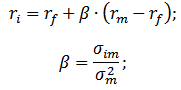 where: r i is the expected return on the stock (discount rate);
r f - profitability on a risk-free asset (for example: government bonds);
r m is the market yield, which can be taken as the average return on the index (MICEX, RTS for Russia, S & P500 for the USA);
β is the beta coefficient. Reflects the riskiness of investments in relation to the market, and shows the sensitivity of changes in stock returns to changes in market returns;
σ im - standard deviation of changes in stock returns depending on changes in market returns;
σ 2 m is the variance of market returns.
Advantages and Disadvantages of CAPM Capital Assets Valuation Model
- The model is based on the fundamental principle of linking stock returns to market risk, which is its advantage;
- The model includes only one factor (market risk) for assessing future stock returns. Researchers such as J. Fam, C. French, and others have introduced additional parameters into the CAPM model to increase its forecast accuracy.
- The model does not take into account taxes, transaction costs, stock market opacity, etc.
Discount rate calculation using the modified CAPM model
The main drawback of the CAPM model is that it is one-factor. Therefore, the modified model for assessing capital assets also includes adjustments for unsystematic risk. Unsystematic risk is also called specific risk, which appears only under certain conditions. Modified Calculation Model CAPM Formula (ModifiedCapitalAssetPricingModel,MCAPM) is as follows:
![]() where: r i is the expected return on the stock (discount rate); r f is the return on a risk-free asset (for example, government bonds); r m –market profitability; β is the beta coefficient; σ im - standard deviation of changes in stock returns from changes in market returns; σ 2 m is the variance of market returns;
where: r i is the expected return on the stock (discount rate); r f is the return on a risk-free asset (for example, government bonds); r m –market profitability; β is the beta coefficient; σ im - standard deviation of changes in stock returns from changes in market returns; σ 2 m is the variance of market returns;
r u - risk premium, which includes unsystematic risk of the company.
To assess specific risks, experts are usually used, because they are difficult to formalize using statistics. The table below shows the various risk adjustments ⇓.
| Specific risks | Risk adjustment,% |
| State influence on tariffs | 0,4% |
| Change in prices for raw materials, materials, energy, components, rent | 0,2% |
| Management risk of the owner / shareholders | 0,2% |
| Key Supplier Impact | 0,3% |
| The influence of seasonality of demand for products | 0,4% |
| Terms of raising capital | 0,3% |
| Total, specific risk adjustment: | 1,8% |
For example, we calculate the discount rate as amended, so if the yield on the CAPM model is 10%, then, taking into account risk adjustments, the discount rate will be 11.8%. Using a modified model allows you to more accurately determine the future rate of return.
Calculation of the discount rate according to the model of E. Famy and C. French
One of the modifications of the CAPM model was the three-factor model of E. Fama and C. French (1992), which began to take into account two more parameters that affect the future rate of return: company size and industry specifics. The following is the formula for a three-factor model of E. Fama and C. French:
where: r is the discount rate; r f is the risk-free rate; r m - market portfolio return;
SMB t is the difference between the returns of the weighted average stock portfolios of small and large capitalization;
HML t is the difference between the returns of weighted average stock portfolios with large and small ratios of book value to market value;
β, si, h i - coefficients that indicate the influence of the parameters r i, r m, r f on the profitability of the i-th asset;
γ is the expected return on the asset in the absence of the influence of 3 risk factors on it.
Calculation of the discount rate based on the model of M. Karhat
The three-factor model of E. Fama and C. French was modified by M. Carhart (1997) by introducing a fourth parameter to assess possible future stock returns - the moment. The moment reflects the rate of price change for a certain historical period of time, when the fourth parameter is used in the model for evaluating the stock's return in the future, it is taken into account that the rate of price change also affects the future rate of return. Below is the formula for calculating the discount rate according to the model of M. Carhart:
where: r is the discount rate; WMLt - moment, rate of change in stock value for the previous period.
Calculation of the discount rate based on the Gordon model
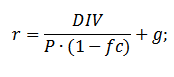
Another method of calculating the discount rate is to use the Gordon model (Continuous Growth Dividend Model). This method has some restrictions on use, because in order to estimate the discount rate it is necessary for the company to issue ordinary shares with dividend payments. The following is the formula for calculating the cost of equity of the enterprise (discount rate):
 where:
DIV - the amount of expected dividend payments per share for the year;
P is the share price;
fc is the cost of issuing shares;
g is the growth rate of dividends.
Calculation of the discount rate based on the weighted average cost of capital WACC
The method of estimating the discount rate based on the weighted average cost of capital (WACC, Weighted Average Cost of Capital) one of the most popular and shows the rate of return that should be paid for the use of investment capital. Investment capital may consist of two sources of financing: equity and debt. Often, WACC is used both in financial and in investment analysis to assess future investment returns, taking into account the initial conditions for the return (profitability) of investment capital. The economic meaning of calculating the weighted average cost of capital is to calculate the minimum acceptable level of profitability (profitability, profitability) of a project. This indicator is used to assess investments in an existing project. The formula for calculating the weighted average cost of capital is as follows:
![]()
where: r e, r d - the expected (required) return on equity and borrowed, respectively;
E / V, D / V - share of equity and borrowed capital. The sum of the actual and borrowed capital forms the capital of the company (V \u003d E + D);
t– income tax rate.
Calculation of the discount rate based on return on equity
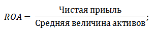
The advantages of this method are the ability to calculate the discount rate for enterprises that are not quoted on the stock market. Therefore, to assess the discount, indicators of return on equity and borrowed capital are used. These indicators are easily calculated on balance sheet items. If the company has both its own and borrowed capital, then the indicator is used - return on assets (Return On Assets, ROA). The formula for calculating the profitability ratio of assets is presented below:
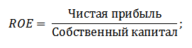
The next of the methods of estimating the discount rate through return on equity (Return On Equity, ROE), which shows the effectiveness / profitability of the capital management of the enterprise (company). The profitability ratio shows what rate of return the company creates at the expense of its capital. The formula for calculating the coefficient is as follows:
Developing this approach in assessing the discount rate through evaluating the profitability of the enterprise as a criterion for assessing the rate, you can use a more accurate indicator - return on capital employed (ROCE,ReturnOnCapitalEmployed). This indicator, in contrast to ROE, uses long-term liabilities (through shares). This indicator can be used for companies that have preferred stocks on the stock market. If the company does not have them, then the ROE is equal to ROCE. The indicator is calculated by the formula:
Another kind of return on equity ratio is ROACE average return on equity (Return on Average Capital Employed).
In fact, this indicator corresponds to ROCE, its main difference lies in averaging the cost of capital employed (Equity + long-term liabilities) at the beginning and end of the estimated period. The formula for calculating this indicator:
ROACE can often replace ROCE, for example, in the EVA Economic Value Added Formula. Here is an analysis of the appropriateness of using profitability ratios to estimate the discount rate ⇓.
Calculation of the discount rate based on expert judgment
If you need to estimate the discount rate for a venture project, then using the CAPM methods, the Gordon model and the WACC is not possible, therefore, experts use to calculate the rates. The essence of expert analysis is a subjective assessment of various macro, meso and micro factors affecting the future rate of return. Factors that have a strong influence on the discount rate: country risk, industry risk, production risk, seasonal risk, management risk, etc. For each individual project, experts identify their most significant risks and evaluate them using point estimates. The advantage of this method is the ability to take into account all the possible requirements of the investor.
Discount rate calculation based on market multiples
This method is widely used to calculate the discount rate for enterprises that have issues of ordinary shares in the stock market. As a result, the market multiplier E / P is calculated, which translates as EBIDA / Price. The advantages of this approach are that the formula reflects industry risks when evaluating the company.
Calculating a discount rate based on risk premiums
The discount rate is calculated as the sum of the risk-free interest rate, inflation and risk premium. As a rule, this method of estimating the discount rate is carried out for various investment projects where it is difficult to statistically evaluate the magnitude of the possible risk / return. The formula for calculating the discount rate taking into account the risk premium:
![]() where:
where:
r is the discount rate;
r f - risk-free interest rate;
r p is the risk premium;
I is the percentage of inflation.
The discount rate formula consists of the sum of the risk-free interest rate, inflation and risk premium. Inflation was highlighted as a separate parameter, because the depreciation of money is ongoing, this is one of the most important laws of the functioning of the economy. Let us consider separately how each of these components can be evaluated.
Methods for estimating a risk-free interest rate
To assess risk-free use such financial instruments that give profitability at zero risk, that is, absolutely reliable. In reality, no tool can be considered absolutely reliable, just the probability of losing money when investing in it is extremely small. Consider two methods for assessing the risk-free rate:
- Profitability on risk-free government bonds (T-bills - state short-term coupon-free bonds, OFZ - federal loan bonds) issued by the Ministry of Finance of the Russian Federation. Government bonds have a maximum reliability rating, so they can be used to calculate the risk-free interest rate. The yield on these types of bonds can be viewed on the CBR website (cbr.ru) and on average it can be taken as 6% per annum.
- Yield on 30-year US bond loans. The average yield on these financial instruments is 5%.
Risk premium assessment methods
The next component of the formula is the risk premium. Since risks always exist, their influence on the discount rate should be evaluated. There are many methods for assessing additional investment risks, we will consider some of them.
Methodology for assessing risk adjustments from Alt-Invest
The Alt-Invest methodology includes the following types of risks in the risk adjustment, presented in table ⇓.
Methodology of the Government of the Russian Federation No. 1470 (dated 11/22/97) estimating the discount rate for investment projects
The purpose of this methodology is the assessment of investment projects for public investment. The specific risk and the correction for them will be calculated through an expert assessment. To calculate the base (risk-free) discount rate, the Central Bank of the Russian Federation refinancing rate was used; this rate can be viewed on the official website of the Central Bank of the Russian Federation (cbr.ru). Specific project risks are assessed by experts in the ranges presented. The maximum discount rate for this method will be 61%.
| Risk-free interest rate | |
| WITH refinancing Bank of the Central Bank of the Russian Federation | 11% |
| Risk premium | |
| Specific risks | Risk adjustment,% |
| Investments to intensify production | 3-5% |
| Product sales increase | 8-10% |
| The risk of market promotion of a new type of product | 13-15% |
| Research costs | 18-20% |
The method of calculating the discount rate Vilensky P.L., Livshitsa V.N., Smolyaka S.A.
| Specific risks | Risk adjustment,% |
| 1. The need for R&D (with previously unknown results) by specialized research and (or) design organizations: | |
| r&D duration less than 1 year | 3-6% |
| r&D duration over 1 year: | |
| a) R&D is carried out by one specialized organization | 7-15% |
| b) R&D is comprehensive and carried out by several specialized organizations | 11-20% |
| 2. Characteristics of the technology used: | |
| Traditional | 0% |
| New | 2-5% |
| 3. Uncertainty of volumes of demand and prices for manufactured products: | |
| existing | 0-5% |
| New | 5-10% |
| 4. The instability (cyclicality, seasonality) of production and demand | 0-3% |
| 5. Uncertainty of the external environment during the implementation of the project (mining, geological, climatic and other natural conditions, aggressiveness of the external environment, etc.) | 0-5% |
| 6. Uncertainty of the development process of the applied equipment or technology. The ability of participants to enforce technological discipline | 0-4% |
Methodology for calculating the discount rate of Y. Honko for various investment classes
Scientists Y. Honko presented a methodology for calculating risk premiums for various classes of investments / investment projects. These risk premiums are presented in aggregated form, and the investor needs to choose the purpose of the investment and, in accordance with it, the risk adjustment. The following are aggregated risk adjustments based on the purpose of the investment. As you can see, with increasing risk, the ability of the enterprise / company to enter new markets, expand production and increase competitiveness also increases.
Summary
In the article, we examined 10 methods for estimating the discount rate that use a different approach and assumptions in the calculation. The discount rate is one of the central concepts in investment analysis, it is used to calculate indicators like: NPV, DPP, DPI, EVA, MVA, etc. It is used in assessing the value of investment objects, stocks, investment projects, management decisions. When choosing an assessment method, it is necessary to take into account the purpose of the assessment and what are the initial conditions. This will allow the most accurate assessment. Thank you for your attention, Ivan Zhdanov was with you.
The discount rate is the rate of return. The indicator affects both the decision to invest, and the assessment of a company or a particular type of business. We calculate the discount rate by several methods and give recommendations in order to prevent errors in the calculations.
What is the discount rate in simple words?
Discounting is the determination of the value of cash flows relating to future periods (future income at the moment). For a correct assessment of future income, you need to know the forecast values \u200b\u200bof revenue, expenses, investments, , the residual value of the property, as well as the discount rate that is used to evaluate the effectiveness of investments.
From an economic point of view - This is the rate of return on invested capital required by the investor. In other words, with its help it is possible to determine the amount that the investor will have to pay today for the right to receive estimated income in the future. Therefore, the adoption of key decisions depends on the value of the indicator, including when choosing an investment project.
Example
When implementing Project A, the investor receives a profit of 500 rubles at the end of the year for three years. When implementing Project B, the investor receives income at the end of the first and at the end of the second year at 300 rubles, and at the end of the third year - 1100 rubles. An investor needs to choose one of these projects.Suppose that the investor has set the rate at 25% per annum. The current value (NPV) of projects “A” and “B” is calculated as follows:
where P k - cash flows for the period from 1st to nth years;
r - discount rate - 25%;
I - initial investment - 500.
NPV A \u003d - 500 \u003d 476 rubles .;
NPV B \u003d - 500 \u003d 495.2 rubles.
Thus, the investor will choose project “B”. However, if he sets a discounted rate, for example, equal to 35% per annum, then the current costs of projects A and B will be 347.9 and 333.9 rubles. accordingly (the calculation is similar to the previous one). In this case, the project “A” is more preferable for the investor.
Therefore, the investor’s decision completely depends on the value of the indicator if it is more than 30.28% (with this value NPV A \u003d NPV B), then project “A” is preferable, if less, then project “B” will be more profitable.
VIDEO: How to calculate net present value in Excel
There are various methods for calculating the discount rate. Consider the main ones in descending order of objectivity.
CAPM Discount Rate Calculation
To calculate the discount rate, the Capital Assets Pricing Model (CAPM) method, which is based on the company's capital assessment, works most effectively and accurately in practice. For more information on how to use the CAPM method for calculation, we describe in the material of the journal "Financial Director".
Determination of the weighted average cost of capital
Most often in investment calculations, the discount rate is defined as weighted average cost of capital (weighted average cost of capital - WACC), which takes into account the cost and the cost of borrowed funds. This is the most objective calculation method. Its only drawback is that in practice not all enterprises can use it (this will be discussed below).
Calculation of the cost of equity
For determining cost of equity a valuation model for long-term assets ( capital assets pricing model - CAPM).
The discount rate (return) on equity (Re) is calculated by the formula:
R e \u003d R f + B (R m - R f),
where R f is the risk-free rate of return;
B - coefficient determining the change in the price of stocks of a company compared to changes in stock prices for all companies in a given market segment;
(R m - R f) - premium for market risk;
R m - the average market rate of return on the stock market.
Let us consider in detail each of the elements of the valuation model of long-term assets.
The rate of return on investments in risk-free assets (R f). As risk-free assets are usually considered government securities. In Russia, these are Russia-30 Eurobonds with a maturity of 30 years.
Coefficient B. This coefficient reflects the sensitivity of the profitability indicators of securities of a particular company to changes in market (systematic) risk. If B \u003d 1, then the fluctuations in the stock prices of this company fully coincide with the fluctuations of the market as a whole. If B \u003d 1.2, then we can expect that in case of a general rise in the market, the stock price of this company will grow 20% faster than the market as a whole. Conversely, in the event of a general fall, the value of its shares will decline 20% faster than the market as a whole.
In Russia, information on the values \u200b\u200bof B-ratios of companies whose shares are most liquid can be found in the information releases of the AK & M rating agency, as well as on its website in the Ratings section. In addition, B-ratios are calculated by the analytical services of investment companies and large consulting firms, such as Deloitte and Touche CIS.
Market risk premium (R m - R f). This is the amount by which the average market rate of return on the stock market exceeded the rate of return on risk-free securities for a long time. It is calculated on the basis of statistics on market premiums over a long period. According to Ibbotson Associates, the long-term expected market premium based on data on the difference between the arithmetic average income in the stock market and the risk-free return on investments in the USA from 1926 to 2000 is 7.76%. Russian companies can also use this value for calculations (in some textbooks, the market risk premium is assumed to be 5%).
WACC calculation
If not only equity, but also borrowed capital is attracted to finance a project, then the profitability of such a project should compensate not only for the risks associated with investing own funds, but also the costs of attracting borrowed capital. To take into account the cost of both equity and borrowed funds, the weighted average cost of capital index (WACC) allows, which is calculated by the formula:
WACC \u003d R e (E / V) + R d (D / V) (1 - t c),
where R e is the rate of return on equity (equity) capital, calculated, as a rule, using the CAPM model;
E is the market value of own equity. It is calculated as the product of the total number of ordinary shares of the company and the price of one share;
D is the market value of borrowed capital. In practice, it is often determined from the financial statements as the amount of the company's loans. If this data cannot be obtained, then available information on the ratio of equity and borrowed capital of similar companies is used;
V \u003d E + D - the total market value of the loans of the company and its share capital;
R d is the rate of return on borrowed capital of the company (the cost of raising borrowed capital). As such costs are considered interest on bank loans and corporate bonds of the company. At the same time, the cost of borrowed capital is adjusted taking into account the income tax rate. The meaning of the adjustment is that the interest on servicing loans and borrowings relates to the cost of production, thereby reducing the tax base for income tax;
t c - income tax rate.
Example
We calculate the rate using the weighted average cost of capital (WACC) model for Norilsk Nickel taking into account current conditions in the Russian economy.
In the calculations we will use the following data as of mid-February:
Rf \u003d 8.5% (rate on Russian European bonds);
B \u003d 0.92 (for the company Norilsk Nickel, according to the rating agency AK & M);
(Rm - Rf) \u003d 7.76% (according to Ibbotson Associates).
Thus, the return on equity is equal to:
Re \u003d 8.5% + 0.92 × 7.76% \u003d 15.64%.
E / V \u003d \u200b\u200b81% - the share of the market value of equity (E) in the total cost of capital (V) of Norilsk Nickel (according to the author).
Rd \u003d 11% - weighted average cost of borrowing for Norilsk Nickel (according to the author).
D / V \u003d \u200b\u200b19% - the share of the company's borrowed capital (D) in the total cost of capital (V).
tc \u003d 24% - income tax rate.
Thus, WACC \u003d 81% × 15.64% + 19% × 11% × (1 - 0.24) \u003d 14.26%.
As we have already noted, not all enterprises can use the approach described above. Firstly, it is not applicable to companies that are not open joint stock companies, therefore, their shares are not traded on stock markets. Secondly, firms that do not have enough statistics to calculate their B-factor, and also are not able to find an analogue company, whose B-coefficient they could use in their own calculations, will not be able to apply this method. Such companies should use other calculation methods to determine the discount rate.
Risk premium assessment method
One of the most common methods of determining the discount rate in practice is the cumulative method of assessing the risk premium. The basis of this method is the assumption that:
- if the investments were risk-free, then investors would demand risk-free returns on their capital (that is, the rate of return corresponding to the rate of return on investments in risk-free assets);
- the higher the investor assesses the risk of the project, the higher demands it makes on its profitability.
Based on these assumptions, the calculation must take into account the so-called "risk premium". Accordingly, the formula will look as follows:
R \u003d Rf + R1 + ... + Rn
where R is the discount rate;
Rf - risk-free rate of return;
R1 + ... + Rn - risk premiums for various risk factors.
The presence of a particular risk factor and the significance of each risk premium in practice are determined by experts.
Expert Discount Rate Determination
The easiest way to determine the discount rate, which is used in practice, is to determine it expertly or based on the requirements of the investor. The approximate value of the corrections for the risk of not receiving the income provided by the project is presented in Table 1.
Table 1. Amendments to the risk of non-receipt of project revenue
However, it should be borne in mind that the expert method will give the least accurate results and may lead to a distortion of the results of project evaluations. Therefore, when determining the indicator by expert method or by the cumulative method, it is necessary to analyze the sensitivity of the project to a change in the discount rate. Then the investor will be able to more accurately assess the risks and its effectiveness.
Example
Consider the conditional projects “A” and “B” from the first example. The results of the analysis of their sensitivity to changes in the discount rate are presented in table. 2.
table 2. Project Sensitivity Analysis
There are other alternative approaches to calculation, for example, using the theory of arbitrage pricing or a dividend growth model. However, these theories are quite complex and rarely applied in practice; therefore, they are not considered in this article.
Practical Application Issues
When calculating, one must not forget to take into account a number of important points. Otherwise, there is a danger of making mistakes.
The volatility of the capital structure. During the calculation period of the project, the structure may change (for example, as the loan is paid, the debt decreases and at some point it becomes zero). Hence the question: how to calculate the discount rate in such a situation?
To determine a single discount rate for the entire period of the project, I propose to use the optimal capital structure. That is, the optimal ratio of own and borrowed funds, at which the cost of capital (WACC) is minimal. But it is important not to forget that in practice the cost of equity is higher than borrowed, therefore, with an increase in the share of borrowed funds, WACC decreases. However, as debt obligations grow, the risk of bankruptcy increases and, accordingly, debt servicing costs increase, and the cost of borrowed capital grows. Accordingly, upon reaching a certain level of the ratio of borrowed to own funds, WACC also begins to grow.
Inconsistency of income tax. When determining the cost of capital, taking into account the tax shield, sometimes you are faced with the problem of choosing the estimated income tax rate. If during the settlement period the company operates under one of the standard tax regimes, then no questions arise - the tax rate established by law is selected. However, there are cases when the income tax rate is variable. For example, when during a certain period of time a project is taxed at a reduced rate (most often during the period of repayment of borrowed funds or during the first years of implementation). In this situation, two calculation options can be distinguished.
1. If one rate (for example, a preferential one) is valid at the beginning of the project and then for a significant part of the time of its implementation (more than half), then you can take it for calculation.
2. If the rate periodically changes and does not remain at the same level for a long time within the billing period, it is necessary to calculate its weighted average value by the formula:

t - project implementation period;
T1, T2, ..., TN - current income tax rates over time periods.
If the company has several separate divisions that fall under the tax laws of various countries, then the rate should be calculated as a weighted average based on several rates and the amount of tax base.

where T is the weighted average income tax rate;
p - the total profit of the enterprise (profit values \u200b\u200bare recommended to be taken for the entire implementation period);
T1, T2, ..., TN - current income tax rates in the territories of various countries;
p1, p2, ..., pN - profit in various countries (for calculation it is recommended to take data for the entire implementation period).
Accounting for inflation. If the project is calculated at prices adjusted for inflation, then inflation is added to the nominal discount rate. It can be taken into account in two ways. First: when the rate is calculated for each step of discounting separately, the forecast value of inflation at this time section is added. Second: in the case of calculating a flat rate for the entire period of the project calculation, the average value of the forecast inflation rate for the project calculation period is added.
Summing up, we note that most enterprises in the process of work are faced with the need to determine the discount rate. Therefore, it should be remembered that the most accurate value of this indicator can be obtained using the WACC method, while the remaining methods give a significant error.
Discounting from English "discounting" - bringing economic values \u200b\u200bfor different periods of time to a given period of time.
If you do not have an economic or financial background, then this term is most likely not familiar to you and this definition is unlikely to explain the essence of “discounting”, but rather it will confuse it even more.
However, it makes sense for the prudent owner of his budget to understand this issue, since each person finds himself in a situation of “discounting” much more often than it seems at first glance.
Discounting - Wikipedia information

Description of discounting in simple words
What Russian is not familiar with the phrase “know the value of money”? This phrase comes to mind as soon as the line at the checkout comes up, and the buyer once again looks at his grocery basket to remove “unnecessary” goods from it. Indeed, in our time we have to be prudent and economical.
Discounting is often understood as an economic indicator that determines the purchasing power of money, its value after a certain period of time. Discounting allows you to calculate the amount that you need to invest today in order to receive estimated income after some time.
Discounting - as a tool for forecasting future profits - is in demand among business representatives at the stage of planning results (profits) from investment projects. Future results can be announced at the beginning of the project or during the implementation of its subsequent stages. To do this, the specified indicators are multiplied by the discount coefficient.
Discounting also "works" in the interests of an ordinary person who is not connected with the world of large investments.
For example, all parents strive to give their child a good education, and, as you know, it can cost a lot of money. Not everyone has financial resources at the time of receipt (cash reserve), so many parents are thinking about a “stash” (a certain amount of money spent by the cash register of the family budget), which can help out at X.
Suppose in five years your child graduates from high school and decides to enter a prestigious European university. Preparatory courses at this university cost $ 2,500. You are not sure that you can cut this money out of the family budget without prejudice to the interests of all family members. There is a way out - you need to open a deposit in the bank, for this to begin it would be nice to calculate the amount of the deposit that you must open in the bank now, in order to receive 2500 per hour X (that is, five years later), provided that the maximum profitable percentage that can offer a bank, say –10%. To determine how much future spending (cash flow) costs today, we make a simple calculation: We divide 2500 dollars into (1.10) 2 and we receive 2066 dollars. This is the discount.
Simply put, if you want to know what is the value of the amount of money that you will receive or plan to spend in the future, then you should “discount” this future amount (income) at the interest rate offered by the bank. This rate is also called the "discount rate."
In our example, the discount rate is 10%, $ 2500 is the amount of the payment (or cash outflow) after 5 years, and $ 2066 is the discounted value of the future cash flow.

Discount formulas
All over the world, it is customary to use special English-language terms to indicate current (discounted) and future value: future value (FV) and present value (PV). It turns out that $ 2,500 is FV, \u200b\u200bthat is, the value of money in the future, and $ 2,066 is PV, that is, the value at a given time.
The formula for calculating the discounted value for our example looks like this: 2500 * 1 / (1 + R) n \u003d 2066.
General discount formula: PV \u003d FV * 1 / (1 + R) n
- The coefficient by which the future value is multiplied 1 / (1 + R) n, called the "discount factor",
- R - interest rate
- N - the number of years from a date in the future to the present.
As you can see, these mathematical calculations are not so complicated and not only for bankers. In principle, you can give up on all these figures and calculations, the main thing is to grasp the essence of the process.
Discounting is the path of cash flow from the future to the present day - that is, we go from the amount we want to receive after a certain amount of time to the amount we have to spend (invest) today.
Life formula: time + money
Let's imagine one more situation that everyone knows: you had “free” money and you came to the bank to make a deposit of, say, $ 2,000. Today, $ 2,000 put into the bank at a bank rate of 10% tomorrow will cost $ 2,200, that is, $ 2,000 + interest on the deposit 200 (=2000*10%) . It turns out that in a year you can get $ 2,200.
If we present this result in the form of a mathematical formula, then we have: $2000*(1+10%) or $2000*(1,10) = $2200 .
If you deposit $ 2,000 for a period of two years, this amount is converted to $ 2,420. We consider: $ 2,000 + interest that accrued for the first year $ 200 + interest for the second year $220 = 2200*10% .
The general formula for increasing the contribution (without additional contributions) for two years looks like this: (2000*1,10)*1,10 = 2420
If you want to extend the term of the deposit, then your income on the deposit will increase even more. To find out the amount that the bank will pay you in a year, two or, say, five years, you need to multiply the deposit amount with a multiplier: (1 + R) N.
Wherein:
- R - this is the interest rate expressed in fractions of a unit (10% \u003d 0.1),
- N - indicates the number of years.
Discount and accrual transactions
Thus, it is possible to determine the contribution at any time point in the future.
The calculation of the future value of money is called “build-up”.
The essence of this process can be explained by the example of the well-known expression “time is money”, that is, over time, the monetary contribution grows due to an increase in annual interest. The whole modern banking system works on this principle, where time is money.
When we discount, we move from the future to the present day, and when we “build up”, the trajectory of the movement of money is directed from today to the future.
Both “calculation chains” (both discounting and accumulation) allow us to analyze possible changes in the value of money over time.
Cash flow discounting method
We have already mentioned that discounting - as a tool for forecasting future profits - is necessary for calculating the assessment of project effectiveness.
So, when assessing the market value of a business, it is customary to take into account only that part of capital that is capable of generating income in the future. At the same time, many points are important for the business owner, for example, the time of receipt of income (monthly, quarterly, at the end of the year, etc.); what risks may arise in connection with profitability, etc. These and other features that affect the assessment of the business, takes into account the method of DDP.
Discount coefficient
The method of discounting cash flows is based on the law on the “falling” value of money. This means that over time the money "cheaper", that is, lose in price compared to the current value.
From this it follows that it is necessary to build on the assessment at the current moment, and all subsequent cash flows or outflows must be correlated with today. This will require a discount factor (Cd), which is necessary to bring future income to its present value by multiplying Cd by payment flows. The calculation formula looks like this:

where: r - discount rate, i - time period number.
DDP calculation formula

The discount rate is the main component of the DDP formula. It shows what size (norm) of profit a business partner can count on when investing in a project. The discount rate takes into account various factors, depending on the valuation subject, and may include: the inflation component, the assessment of capital shares, the return on risk-free assets, the refinancing rate, the interest on bank deposits and more.
It is generally accepted that a potential investor will not invest in a project whose value will be higher than the present value of project income in the future. Similarly, the owner will not sell his business at a price that is less than the estimated value of future income. Based on the results of the negotiations, the parties will agree on a market price that is equivalent to the current value of projected income.
The ideal situation for the investor is when the internal rate of return (discount rate) of the project is higher than the costs associated with finding financing for a business idea. In this case, the investor will be able to "earn" as banks do, that is, accumulate money at a reduced interest rate, and invest it in the project at a higher rate.

Discounting and investment projects
The cash flow discounting method meets the investment motives of the business.
This means that the investor who invests in the project does not acquire technical or human resources in the form of a team of highly qualified specialists, modern offices, warehouses, high-tech equipment, etc., but the future flow of money. If we continue this thought, it turns out that any business “launches” the only product on the market - it is money.
The main advantage of the cash flow discounting method is that this valuation method, the only one of all existing ones, is focused on the future development of the market, which contributes to the development of the investment process.
One of the most important criteria for evaluating an investment project is the discount factor. High-quality business planning involves mandatory accounting for changes in the value of money over time, so all future cash flows should be brought to their current state. Let us dwell in more detail on what a discount coefficient is and how to determine its value.
The concept of discount coefficient and its value
Cash flow discounting coefficient is a digital indicator, using which you can understand how much money you can get after a certain time, taking into account the time factor and possible risk. Thus, the cash flows in the future are brought to the state on the day of analysis.
In business designing, “money now” is always preferable than “money later”, because they can be invested in another business and receive income or placed on a bank deposit and receive a fixed percentage. Therefore, before investing, the investor must be sure that during the life cycle of the project he will not only not lose from the cheapening of money, but will also be able to make a profit.
The time interval during which the initiative is realized and brings profit to the participants is set in advance. As a rule, it is determined by the regulatory terms for the use of installed equipment, after which the technical capabilities of the production are exhausted. The objectivity of calculations largely depends on the correct determination of the time frame of the undertaking.
The value of the discount coefficient is used in different situations:
- assessment of the effectiveness of the economic activity of any company;
- calculation of the effectiveness of the investment project;
- consideration of alternative investment options both between different initiatives and within the same enterprise (choosing the most promising development path);
- multilateral settlements and lending.
This indicator actually establishes a certain standard of costs or capital inflows when investing in another undertaking. In other words, the coefficient (or factor) makes it possible to determine the amount of interest by which the expected income should be multiplied in order to reach a specific amount in relation to the current state.
The method of determining the value of the indicator
Let us consider in more detail how to calculate the discount coefficient. Usually, we are talking about a multi-step calculation of the prospects and economic efficiency of an investment undertaking, therefore, it leads the flow volume at the nth step to the time of reduction.
The total cash flow is as follows:
PV \u003d FV * 1 / (1 + R) n
- PV is the present value;
- FV is the future value.
In this formula, a component is determined that determines the magnitude of the reduction factor. Actually, the formula for calculating the discount coefficient looks like this:
KD \u003d 1 / (1 + R) n
wherein:
- R is the set value;
- n is the number of periods (steps), which is the number of years (months) from the future to the current moment.
The resulting indicator always has a value of less than one. It shows the value of one invested monetary unit (ruble, euro, dollar) after a certain time, subject to the conditions that are accepted for calculation.
The most important component for calculating the coefficient is the discount rate, which is also called the discount rate. For its definitions, there are a number of techniques based on various principles:
- dividend method (Gordon model);
- the cost of capital assets of the enterprise (CAPM model and its many modifications);
- availability of borrowed and own funds (WACC model);
- return on equity method (ROE, ROA, ROACE, ROCE);
- method of calculating risk premiums (cumulative);
- expert method based on subjective forecasts of specialists.
 The rate of inflation, the value of long-term deposits or loans, the size of the Central Bank, etc. can be taken as the discount rate. In any case, what this criterion will be, the investor decides at his own risk. If the discount rate is set incorrectly or it does not take into account all the main risks, then the reduction factor will be incorrect. This will give the investor an incorrect forecast, which could lead to losses.
Another component of the formula is the life cycle of the undertaking, that is, the number of periods under consideration during which the project will generate. The more precisely these two introductory ones are established, the more accurate the final result will be.
Examples of calculating cash flows using a discount factor
Let's consider an example of calculation. A businessman is investing 800 thousand rubles in a new six-year project. According to the business plan presented by the initiator, in 6 years he will be able to receive 1.5 million rubles in a one-time payment. The cumulative method determines the discount rate of 12%, while the percentage of the discount rate is recorded in the calculation as a part of unity (0.12). Now, using the standard formula, we can calculate the magnitude of the factor:
Kd \u003d 1 / (1 + 0,12) 6
Kd \u003d 1 / 1,9738
Kd \u003d 0,5066
We got a cast factor of 0.5066. After that, the discounted formula calculates the indicators of the value of the reduced cash flow:
PV \u003d FV * 1 / (1 + R) n.
PV \u003d 1500000 * 0.5066
PV \u003d 759900
From the result obtained, it can be concluded that the investor is disappointing that, under such starting conditions, he should not expect not only profit, but even a simple return on invested money. Therefore, such a proposal should be rejected or proposed to change the basic conditions of the project, if appropriate (shorten the implementation period or reduce the discount rate).
Suppose that the discount rate in our example is reduced to 10%. In this case, the coefficient value will be 0.5645, and the reduced cash flow will increase to 846750 rubles, which will make the project profitable. A similar situation arises if the implementation period is reduced to 5 years at a rate of 12%: the factor will be 0.5674, and the flow will be 851100 rubles.
It should be noted that in order to determine the discount coefficient, there is no need to immerse yourself in mathematical formulas each time. To simplify this task, a table of discount coefficients has been developed and is widely used in practice. It is built according to the standard scheme, like the tables of Pythagoras or Bradis, that is, the sizes of interest rates are indicated on one axis, and time periods on the other. To find the desired indicator, it is enough to find the cell where they intersect, it contains the value of the coefficient accurate to ten thousandths (up to the fourth decimal place). 
All of the above coefficient values \u200b\u200bare taken from this table. This significantly speeds up the calculations and makes it possible to calculate alternative scenarios of events without unnecessary efforts.
We considered the task in which the payment of money was provided in one payment after the end of the project. In practice, situations where payments are made annually are much more common. Then, for the calculation to be correct, it is necessary to find the reduction coefficient for each year separately. For example, our investor will receive his and a half million for 6 years of the initiative’s life cycle at a discount rate of 10% in equal parts of 250 thousand rubles per year (i.e. as annuity):
Using the formula for annual calculations, you can find the coefficients separately for each period, and then sum them up:
| CF 1 | CF 2 | CF N | |||
| NPV \u003d | ----- | + | ------ | +...+ | ------ |
| (1+ R) | (1+ R) 2 | (1+ R) 6 |
PV \u003d 227272 + 206611 + 187828 + 170765 + 155279 + 141083 \u003d 1088838 rubles.
If you use the table of annuity payment ratios, then it will be enough to multiply the size of the average annual payment by the factor indicated in the desired cell of the table (in this case, 4.3553). 
PV \u003d 250000 * 4.3553 \u003d 1088825 rubles
Thus, we see that the indicator found by the formula is almost similar to the value determined using the tables (1088838 versus 1088825).
Some features of practical calculations of the reduction factor
In conclusion, I would like to dwell on a few more points related to bringing cash flows, which are asked by Internet users. In particular, the question arises of how to calculate the factor when the step is set in different units, for example, years and months, and whether the formulas differ in such calculations.
When the discount period is equal to one month, the coefficient is calculated by the following formula:
1 / (1 + R)to the extent (Month - 1) / 12,
- R is the discount rate;
- Month - the number of the ordinal month of the project.
With the annual cast period, the following calculation mechanism is used:
1 / (1 + R)to the extent Year - 1,
- Year - the ordinal number of the life cycle of the undertaking.
If the period is considered quarterly, then for each month of the quarter, the indicator equal to the last month in the quarter is taken into account, that is, for 1, 2 and 3 months, the indicator is 3 months, etc.
Also, forums discuss the situation when regulatory authorities sometimes require to calculate the coefficient of reduction according to the formula KD \u003d 1 / (1+R) ^ (n-0.5) instead of the standard KD \u003d 1 / (1+R) ^ n.
This approach is called the model of average annual discounting. Here discounting is carried out as of the middle of the calendar year (or reduction period), and not at its beginning or end.
Mid-period discounting is applied in cases when there is a constant uniform inflow of money (for example, from the work of an industrial enterprise). Although, among experts, opinions on the advisability of such a calculation method differ.
The discount coefficient, due to its flexibility, is widely used by economists and financiers. It shows the perspective and potential profitability of an individual project in the time period. At the same time, this financial instrument has a serious drawback: it works well in states with stable markets and well-established market mechanisms. Its application in countries that are characterized by a transitional economic model threatens with significant inaccuracies, since it is very difficult to adequately calculate many risks for finding the discount rate in such conditions.