
Valuation of shares with constant dividend growth rates. Valuation of shares based on discounted dividends Average annual growth rate of dividends formula
When an investor buys a share, he generally expects to receive two types of cash flows:
dividends for the holding period,
the expected end-of-ownership price.
To determine expected dividends, assumptions are made about expected future income growth rates and payout ratios. The required return on a stock depends on its risk. Several models for assessing risk and profitability have been developed (CAPM, index models, arbitrage and factor models, etc.).
The dividend discount model (DDM) is a tool for assessing assets (the intrinsic value of a company's shares) in order to identify whether the latter are overvalued or undervalued. O
The dividend discount model (DDM) is a tool for assessing assets (the intrinsic value of a company's shares) in order to identify whether the latter are overvalued or undervalued.
All dividend discount models can be divided into two large groups: deterministic and stochastic. The former reflects the traditional approach to assessing the present value, according to which it is assumed that the flow of future dividend payments is a well-defined value. The second approach was proposed relatively recently. It views the future dividend stream as uncertain. This is an important assumption, since in this case it becomes possible to construct the probabilistic distribution of a random variable of the present value, and, therefore, to find the confidence interval that will determine the significance of the result obtained. This is the main advantage of stochastic dividend models. After receiving any result, it is difficult to say how much you can trust him, and whether the investor should rely on him in his further actions, assuming that the company's shares are really undervalued or vice versa. Thus, these types of models are becoming important for the investment decision-making process.
Deterministic DDM.
As mentioned above, the basis of all DDM is the use of the discounted value method, which implies that the fair price of an asset is the present value of expected future cash flows (in the case of shares, these are dividend payments that will be paid). Basic model has the form
 , (4.99)
where R- theoretical share price;
D t- the expected size of the dividend to be paid in the period t;
r t- the discount rate that corresponds to the level of risk of investing in the shares of the given company.
The basic model considers an endless stream of dividends, making it impossible to calculate value R... In this regard, it is necessary to make a number of assumptions, in particular, about the finiteness of dividend payments. In this case, the dividend flow is estimated over a finite period of time (say, N years), and a certain estimate of the future share price is discounted, which characterizes the reduced post-forecast dividend flow. Equation (4.99) then takes the following form:
where P N is the expected share price at the end of period N, when it is planned to sell it.
With this assumption, it is clearly possible to estimate the flow of future dividends since a reasonable time horizon is considered. However, the question arises of assessing this future value. It also remains uncertain how to account for the time-varying discount rates.
The next assumption is the assumption that the discount rate is constant. In this case, the discount rate r will simply be considered as a weighted average of all rates for the period (this approach is very common, for example, calculating the yield on YTM bonds). Any inaccuracies caused by such an assumption are minimal compared to the errors that can occur when trying to estimate all future discount rates. Taking this into account, equation (4.100) will have the following form:
Now, to calculate the present value, it is necessary to predict or determine the following initial parameters:
expected final price (future value) ( P N);
expected flow of dividends for N years ( D 1 - D N);
discount rate (r).
The hardest part is estimating future value. It represents the present value of all future dividend payments. In practice, this value is usually predicted on the basis of dividends or company income, and then refined based on requirements for profitability, price / earnings ratio and capitalization rate. It should also be borne in mind that P will be negligible and can be neglected in the case when N is very large. As for the discount rate, it is usually determined from the CAPM asset pricing model discussed above.
The next variation of DDM is deterministic model of constant growth. This model assumes that the growth rate of dividends throughout the life of the stock is constant. In turn, this model assumes two more options: an additive growth model (growth in arithmetic progression) and a geometric growth model.
The additive model of constant growth:
 , (4.102)
where d- an increase in the amount of the dividend.
The geometric growth model is as follows:
where g - the estimated growth rate of the dividend, r - the cost of attracting equity capital... Moreover, if N tend to infinity, then we get:
 (4.104)
This model is also known as the model Gordon. If we express the dividend of the next period through the current one, we get:
 (4.105)
The Gordon model is most suitable for firms with growth rates equal to or lower than the growth rate of the economy and with established practice of paying dividends
However, the studies carried out have shown that these models give inadequate results for cases when the growth rates of dividends are far from constant, although they may well be applicable when they approach those. The Gordon model is used to evaluate a firm in a phase of sustainable growth. Dividends and growth rates are maintained indefinitely. The Gordon model also applies to firms with growth rates equal to or below the growth rate of the economy and with established dividend payout practices. Reputable firms pay stable dividends. In the United States, the average payout ratio is 60%. There are three main methods for assessing growth rates:determination of growth rates based on fundamental indicators,
historical growth rates,
assessment by stock analysts.
Methods for assessing historical growth. To assess historical growth, arithmetic and geometric mean models, log-linear regression models, time series models (autoregressive moving average model ARIMA- (Autoregressive integrated moving average)), evaluation by analysts. Analysts use different types of information about the firm. In some cases, their forecasts are better than those based on historical data.
Example 11. Find the value of a share if the following information is available.
Earnings per share in 2000 equal to 3, 13 (EPS).
Dividend payout ratio (  ) = 69.97% (PR).
Dividends per share are 2.19 (  ).
).
The return on equity is 11,635 (ROE).
The cost of raising equity capital is determined using the CAPM model. Let in our case it is equal to  =9%.
=9%.
Solution. The price according to the Gordon model is  .
.
Find g the expected growth rate.
The share price (or the cost of equity) is equal to  .
.
If the shares were sold at a price of 36.59 on the day of the analysis, then they can be considered undervalued.
Example 12. REIT investment funds, established in 1970, are legally entitled to invest in real estate and transfer tax-free profits to investors. In 2000, the fund paid out dividends of 2.12 per share on earnings per share of $ 22.22. Find the value of a share if the average beta for real estate funds is 0.69, the risk-free interest rate is 5.4%, and the risk premium is 4%.
Solution. EPS = $ 22.22; ROE = 12.29%; D 0 = $ 2.12;  = 8.16%. Let's find the dividend payout ratio PR = D 0 / EPS = 2.12 / 22.22 = 0.95. The cost of attracted capital according to CAPM is
  = 5.4 + 4 * 0.69 = 8.16%. The expected growth rates are g = (1- 0.95) * 12.29 = 0.55%.
The share price is  = 2.12 * (1 + 0.55) / (8.16- 0.55) = 28.03 $. If on May 14, 2001, the fund's shares were sold at $ 36.57, then the shares were significantly overvalued.
To calculate the value of a share using a one-phase model, you need to know
Two-phase model.
In the case of long-term investments, models are used that try to account for the life cycle of the stock. The simplest form of such models is two-phase model, within which a period of accelerated growth of dividends and a phase of stable growth rates are considered. This model assumes that high growth rates can be observed only in a limited period of time, after which the company enters a phase of more stable development. Such a model can be described as follows:
 , (4.106)
where  ... The first term of the equation shows, respectively, the size of all dividend payments made during the period of high growth rates, while the second - for the period starting from N + 1 and up to infinity. Exceptional growth rates -
  and stable growth
  .
.
Application of a two-phase model.
 The two-phase model is used for firms with a period of rapid growth. For example, a patented company, a firm operating in an industry experiencing rapid growth, with barriers to entry for other firms. Example from Procter & Gamble. 12 For firms paying dividends as balances cash flows(remaining after the payment of debt, reinvestment).
Model H - two-phase model.
This model assumes that growth rates fall linearly.
Example 13... Two-phase model for P&G. The company faces two challenges. Saturation of the US market, where the company receives half of its revenues. Increased competition. But suppose the company will grow over the next 5 years by expanding into new markets and introducing new products. The company pays high dividends, and has not accumulated significant volumes over the past decade Money... Calculation data are given below.
Equity cost  = 5,4 + 0,85*4 = 8,8%.
The calculation of the expected growth can be carried out using one of the models G = KNP * ROE * (1-PR).
CIT is the ratio of retained earnings, which in this case is assumed to be 25% g = (1- 0.4567) * 0.25 = 13.58%. Beta is estimated to rise to 1, the cost of equity is  = 5,4 + 4*1 = 9,4%.
Let the company's growth rate be equal to the economic growth rate of 5%, and the return on equity will drop to 15% lower than the industry's 17.4%.
KNP = g / ROE = 5/15 = 33.33%. The dividend payout ratio is 1 - 0.3333 = 0.6666.
 (4.107).
The first part of the formula is the present value of the dividend, which is
 7,81$.
The second part is the present value of dividends in the second phase
 59,18$
The share price is P = 7.81 + 59.18 = $ 66.99.
It is alleged that at the time of the analysis on May 14, 2000, P&G shares were sold at a price of $ 63.90, therefore the shares are being sold at a discount.
Three-phase model.
A more complex variation of this model is three-phase model, within which the so-called transitional phase is also considered. It proceeds from the fact that the development of the company is more progressive than abrupt in nature, and therefore a transition period can be distinguished between the phases of high and stable growth rates. The model in this case looks like:
Rice. 4.16. Three-phase model.

 ,
,
The duration of these stages will naturally vary from company to company. Thus, young, fast-growing companies will experience a longer growth phase than mature companies. Interestingly, according to the available data, on average, the growth and transition phases account for up to 25% of the expected income, while the maturity stage accounts for up to 50%. However, this also depends on the policy of the company. Thus, a company with high growth rates and low dividend payments seems to transfer the relative contribution to the stage of maturity, while companies with the opposite situation - to the growth and transition phase.
This model is also known as the E-model (E-earnings-income). The three-phase growth model is widely used by investors, since it allows them to get quite adequate results. For example, it is used by Salomon Brothers.
Stochastic Dividend Discount Models
Stochastic dividend discount models assume that the flow of future dividend payments follows a stochastic process, from which the present value is found. At the same time, processes with the characteristics of Markov movement are considered, which is well suited for temporary payments such as dividends. For the assessment process, the general history is not important - only the current value of the dividend and the probabilistic path of further development of this uncertain process are important. Markov's movement is precisely characterized by the fact that it does not take into account the previous history. These models are divided into two types: binomial (assuming two outcomes) and trinomial (respectively –3 possible outcomes).
Binomial models assume that dividend payments will either remain at the same level or change (in this case, a change in one direction is considered - usually an increase, but neither at once). In turn, they are subdivided into additive and geometric growth models.
The additive stochastic growth model is as follows:
 with probability
  will increase
 with probability
  Will not change
where: d- increase in dividend in cash;
p- the likelihood that the dividend will increase
 (4.109)
It should be noted that this model is also indispensable for a situation where the growth rate of dividends is not constant.
It should be borne in mind that there is always the possibility of bankruptcy of the company. With this in mind, we can calculate some more low level prices:
 with probability R
D t +1 =  with probability
0 with probability 
where p B is the probability of bankruptcy.
 (4.110)
The geometric model looks like this:
D t (1+ g) with probability R
D t +1 =  D t with probability (1-p)
 (4.111)
It is very important that, unlike all previous models, this model can be more or less successfully used in a situation of volatile dividend growth rates. Here you can also determine a lower price level, taking into account the likelihood of the company's bankruptcy:
 (4.112)
Finally, consider the trinomial stochastic model, which is also known as the generalized Markov growth model. It is natural for companies to cut their dividend payments from time to time. This model just allows you to take into account such a scenario. Thus, it assumes three possible outcomes: dividends rise, fall, do not change.
There are also two options for growth: in arithmetic and in geometric progressions.
The additive version of this model is as follows:
Dt + d with probability R U
D t +1 = D t - d with probability R D
D t with probability (1-p U -R D )
where: p U is the probability that the dividend will increase; R D - the probability of a fall in the dividend.
 (4.113)
It is quite obvious that if the probability of reducing the size of dividend payments is equal to zero, then the model is automatically transformed into an equation that characterizes the corresponding binomial model.
Taking into account the probability of bankruptcy, we have:
Consider a geometric model:
Dt (1+ g) with probability R U
D t +1 = D t (1- g) with probability R D
D t with probability ( 1-r U -R D )
 (4.115)
And also taking into account the possible bankruptcy of the company:
 (4.116)
According to the conducted "tests" of these models, trinomial models give more correct estimation results in comparison with binomial ones. As for the choice between using additive or geometric models, there were no advantages here - both types are equal, since for some companies more adequate results were obtained using the former, while for others geometric models were more suitable.
The main advantage of stochastic DDM is the ability to construct the distribution of the value of P, since it is a random variable. This makes it possible to assess how significant the result obtained by using DDM is. However, it is very difficult to determine the type of distribution of this present value, and even more so, its parameters (variance, etc.). Typically, Monte Carlo simulation is used to generate a given distribution and estimate its parameters. Sometimes, however, they start from the assumption that the distribution is normal. In this case, it seems possible to calculate the main characteristics of the distribution. The results are sometimes quite satisfactory and coincide with those obtained by the Monte Carlo method, but this assumption is not justified, therefore, the best option is to use the above method.
Despite the fact that the application of stochastic models has not yet received sufficient application in practice, they give more satisfactory results, and also allow us to conclude about the statistical significance of the models.
A common disadvantage of DDM is, first of all, the problem of evaluating the initial (necessary for calculation) data - how to more accurately determine, for example, the final price? The question remains open. Secondly, it should be understood that DDM speaks only of the relative value of the shares, but does not give any information about when one can expect the beginning of the movement of the market price of a share to its theoretical / intrinsic value. This means that you can buy shares of a certain company, deciding on the basis of the analysis that they are undervalued, and wait a very indefinite period of time before they enter the price. But this is a different question, rather related to the investment strategy.
In general, DDM is a very popular tool among investors, since, being impartial to the influence of the market, it allows obtaining fairly reliable estimates of the company's intrinsic value. However, even more reliable results can be obtained if they are used alongside, for example, with factorial models.
Criticism of the model. The model gives too conservative cost estimates. The model does not include other ways of giving money to shareholders. But it is possible to do this in a modified version of the model.
Discounting model checks. The test of the model is its ability to predict overvalued and undervalued stocks. The research results show that in the long run, the model produces excess returns.
Of the existing methods for assessing the value of a company in a terminal year, consultants-appraisers most often use the Gordon method, which is essentially similar to the approach based on capitalization of income:
GV - the cost in the terminal period - at the end last year forecast period,
Cash flow of the first year of the post-forecast period,
Discount rate for the first year of the post-forecast period,
g - long-term growth rate of cash flow in the terminal forecast period.
A feature of the methods of capitalization and discounting of cash flows is that, as a rule, only one of the methods is used, which is due to the conditions of application of these approaches to valuation.
However, this does not exclude the possibility of calculating the value of a company using two methods simultaneously.
The main prerequisites for using the direct capitalization method are as follows:
The amount of current income is stable, predictable, or changes with constant growth rates, i.e. in the near future, income from the facility will remain at a level close to the current one;
The current activities of a company can provide some insight into its future activities.
The method based on discounted cash flows is more appropriate when a significant change in future income compared to current income is expected, i.e. when the company's activities are expected to differ materially from the current or past.
Particular attention should be paid to companies whose functioning in the future will decline (the growth rate is negative) or whose economic life will cease in the near future (the probability of bankruptcy is high).
In this case, the use of both methods may be questionable.
It should be noted that the approach based on discounting future cash flows relies on events that are only expected. Therefore, the value obtained using this approach directly depends on the forecast accuracy of the appraiser, analyst.
This approach should not be used when there is insufficient data to generate a reasonable forecast of net cash flow for a sufficiently long period in the future.
However, even using rough projections, a discounted future revenue stream approach can be useful in determining the estimated value of a company.
Among other things, it is necessary to take into account the stage of the life cycle of the company and the industry, as well as the type of company being assessed.
It is obvious that the use of the capitalization method at the time of active growth of the company is unlikely to give an adequate cost result.
Examples are telecommunications companies, high-tech business developing robotics, innovative products, companies in the process of restructuring, etc.
In addition, when capitalizing income, it is necessary to understand that for all subsequent periods, not only the amount of the company's income is broadcast, but also the structure of its capital, the rate of return, and the level of risk of the company.
Thus, in order to choose a method for calculating the cost, it is necessary to understand how the company's income or cash flows will change in the near future, to analyze not only financial condition of the evaluated company and the prospects for its development, but also the macroeconomic situation in the world, in the country, in the industry to which the company belongs, as well as in related industries.
Big role the choice of an assessment method is concerned with the purpose of the assessment itself and the intended use of its results.
For example, in the case when it is required to quickly determine the market value of a business using the income approach or to confirm the results obtained by methods within the framework of the comparative or cost approaches, the capitalization method is optimal, since it will quickly get a relatively reliable result.
Also, the capitalization method is justified when preparing analytical materials when a deep immersion in financial flows company or it is not possible.
An almost ideal case for using the capitalization method is the rental business.
In all other cases, especially when the income approach is the only one within which the cost is calculated, the method of discounting cash flows is more preferable, in our opinion.
It is customary to use the Gordon model to calculate the cost of reversion (terminal value) when using the discounted cash flow (DCF) method to determine the value of non-depreciating assets. At its core, the Gordon model formula is the sum of an infinite discounted income stream. The calculated dependence is as follows:
Srev - the cost of the reversion;
CHOD - clean operating income;
Y is the discount rate;
g- the rate of change in CHOD;
m is the number of the initial period;
Abbreviated notation of the formula of the Gordon model.
For depreciating assets such as real estate, the cost of reversion is usually determined by other methods. As one of the calculation options, the method of direct capitalization of the NPR of the first year of the post-forecast period is used. The direct capitalization method (PC) is also used as an independent method for determining the value of real estate objects.
However, unlike the DCF method, the PC method describes a different model of property ownership. This method assumes that the investor, investing in real estate, owns this property until the end of its life and at the same time accumulates funds for the subsequent acquisition, after complete wear and tear, of a similar property. That is, thereby deliberately reduces the amount of incoming income by the rate of return on capital. The dependence for the PC method is as follows:
Co - the cost of the property;
R is the capitalization ratio;
f- the rate of return of capital;
index 0 - corresponds to the evaluation date;
index 1 - corresponds to the first forecast period.
Since the PC and DCF methods reflect slightly different models of investor behavior, it is not surprising that, given certain initial data, they can give different results.
To demonstrate the correctness of the above descriptive model of the PC method, we transform dependence (2) to the following form:
Thus, we have obtained the classic formula for calculating the return on invested capital. For example, in the case of lending - the ratio of annual interest payments on a loan to the amount of the loan.
Since the capital return rate is calculated taking into account the period of the remaining economic life of the object (the period of ownership of capital), it follows that the PC method is based on a model that assumes that the investor, after investing capital in an asset, will own it until the end of its economic life. which confirms the above.
In fairness, it should be noted that the DCF method for a non-depreciating asset that uses the Gordon model (since no return on capital is required) can also be considered a model that assumes infinite ownership of the asset.
Dependence (3) can be written as follows:
If NPR = const (g = 0), the first term in dependence (4) corresponds to the formula of the Gordon model in the absence of a change in NPR. Therefore, substituting formula (1) into (4) and transforming the resulting dependence, we obtain:
Dependency analysis (5) indicates an at first glance unexpected result: a depreciable asset (having a finite life) generates an endless stream of income. This can be explained as follows. Since the PC method assumes the return of capital at the end of the asset's life, to acquire a similar asset, in fact the model described by the PC method assumes infinite ownership of a periodically updated asset with a limited life.
If CHOD const (g 0), then in dependence (5) should be used
Yо is the discount rate for the DCF method.
Transforming dependence (5) for this case, we obtain:
The analysis of dependence (6) allows us to conclude that the methods of PC and DCF in the general case not only reflect different models of investor behavior, but are also characterized by different rates of return, which is quite logical, since different periods of ownership of an object involve different risks.
However, the fact that the rate of return for the PC method with a growing NPR is less than the discount rate for the DCF method, at first glance, does not seem entirely logical, since usually, the longer the asset holding period (asset life), the higher, in general, default risk. This explains, for example, that on stock market the later the maturity of the bond, the higher its yield. However, in the case of a depreciable asset, the opposite effect seems to be observed, due to the fact that over time, as the recovery fund accumulates and the value of the asset decreases, the amount of losses in case of default decreases. Consequently, the integral value of the default risk in this case is lower.
In fact, the idea that when using the PC method, it is necessary to take into account the growth rate of the NPR not only in the numerator, but in the denominator, was expressed, for example, in. However, the absence of an explicit formula led to the fact that in practice this moment was usually not taken into account in the calculations. Apparently, in this regard, the results of the calculation by the PC and DCF methods with the same initial data, in the case of non-constant NPR and the same rates of return, differed, sometimes very significantly, among themselves. Moreover, the result of the PC method, with a growing RRP, was always lower than the result of the DDP method. Taking into account the growth rate of NPR in the denominator makes it possible to reduce this discrepancy in the calculation results. However, differences in results may remain due to initial differences in models. Dependence (6) can also be recommended for use when capitalizing the NPR of the post-forecast period if the DCF method is applied.
Chapter 2. Assessment market value JSC "Kalugapribor" (JSC "Kalugapribor")
In practice, we will consider the Gordon model, analyze the formula and an example of calculation in Excel for real companies.
Gordon's model for business valuation. Formula. Definition.
Gordon's model ( English Gordon growth model) - used to assess the cost of equity and the return on an ordinary share of the company. This model is also called the constant growth dividend model, since the key factor determining the growth of the company's value is the growth rate of its dividend payments. The Gordon model is a variation of the dividend discounting model.
The purpose of evaluating the Gordon model: assessment of the return on equity capital, assessment of the cost of the company's equity capital, assessment of the discount rate for investment projects
The model has a number of limitations on applicability and is used when:
- stable economic situation;
- the product sales market has a large capacity;
- the company has a stable volume of production and sales of products;
- there is free access to financial resources(borrowed capital);
- the growth rate of dividend payments should be less than the discount rate.
In other words, the Gordon Model can be used to evaluate a company if it has sustainable growth, which is expressed in stable cash flows and dividend payments.
Assessment of the return on equity of a company using the Gordon model

You can similarly rewrite the formula for next year's dividend payments by increasing them by the size of the average growth rate.

r is the return on equity of the company (discount rate);
D 1 - dividend payments in the next period (year);
D 1 - dividend payments in the current period (year).
P 0 - share price at the current time (year);
g - average growth rate of dividends.
Evaluation of stock returns based on the Gordon model using the example of Gazprom
An example of evaluating the profitability of a company using the Gordon model in Excel
Let us consider an example of the assessment of the future profitability of OAO Gazprom using the Gordon model. OAO Gazprom was taken for analysis because it is a key national economy, has a variety of sales and production channels, i.e. has a fairly stable vector of development.
At the first stage, it is necessary to obtain data on dividend payments by year. To get statistics on the amount of dividend payments, you can use the "InvestFuture" website and the "Shares" → "Dividends" tab.

Obtaining data on dividends
This is how the period from 2000 to 2013 was taken for the shares of OJSC “Gazprom”. The figure below shows statistics on the amount of dividends per common share.

Data for calculating stock returns according to the Gordon model
It should be noted that for the correct application of the Gordon model, dividend payments must increase exponentially. At the next stage, it is necessary to obtain the current value of OAO Gazprom shares on the stock market; for this, you can use the Finam service.

Determination of the current value of a share of OJSC "Gazprom"
The current value of OAO Gazprom shares is RUB 150.4. Next, let's calculate the average growth rate of dividends and the expected yield.
Average annual growth rate of dividends= (B20 / B7) ^ (1/13) -1
Expected return on stock= B20 * (1 + D7) / E7 + D7
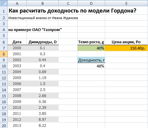
Calculating the expected return on the Gordon model in Excel
The expected return on Gazprom shares for 2014 is expected to be 48%. This model is well applicable for companies with a close relationship between the growth rate of dividends and the value in the stock market. As a rule, this is observed in a stable economy without severe crises. The domestic market is characterized by instability, low liquidity and high volatility, all this leads to the complexity of using the Gordon model to assess the return on equity.
Summary
The Gordon model is an alternative to the CAPM model (capital asset pricing model) and allows you to estimate the future profitability of a company or its value in the market in the context of an overall stable economic growth... Applying the model to emerging capital markets will skew the results. The model can be adequately applied to large national companies from the oil and gas and raw materials industries.
Given the constant growth of dividends with a growth rate of g and a dividend for year C, the price of PV shares can be calculated using the Gordon formula: PV = C * (1 + g) / (r - g)
This model assumes that dividends on shares will grow indefinitely at a constant growth rate. The inclusion of the dividend growth forecast in the previous formula will allow the result to be adjusted for that part of the value for shareholders that is obtained as a result of the reinvestment of profits. The initial assumption is that successful reinvestment will lead in the long term to an additional increase in profits and, accordingly, to an increase in dividends. Mathematically, this model is based on the Gordon model and has the following form:
P =, (7)
where Do is the last actually paid dividend;
r - required rate of return
g is the expected growth rate of the dividend.
The assumption of constant growth in dividends is typical only for mature companies (there are not many of them).
33. Procedure for payment of dividends
The dividend can be paid quarterly, semi-annually or annually (the frequency is regulated by national legislation). The dividend payment procedure adopted in most countries is standard and takes place in several stages (Fig).
Announcement Date - the day when the Board of Directors makes a decision (announces) the payment of dividends, their amount, census and payment dates. The census date is the date of registration of shareholders entitled to receive the declared dividends. The census date is usually set 2-4 weeks before the dividend date. The ex-dividend date is usually set four business days before the dividend census. The payout date is the day the checks are sent to shareholders.
According to Ross. Zak-woo the procedure for payment of dividends is negotiated upon issue valuable papers and is stated on the reverse side of the share or certificate. Shares purchased no later than 30 days before the officially announced date of dividend are entitled to dividend. An interim dividend is declared by the Board of Directors of the joint-stock company per one common share based on the results of the past period. The size of the final dividend per one common share is announced by the general meeting of shareholders based on the results of the year, taking into account the payment of interim dividends. The Board of Directors and general meeting shareholders are prohibited from declaring and paying dividends in the following cases:
a) in annual balance society has losses (until they are covered or reduced authorized capital);
b) the company is insolvent or may become insolvent after the payment of dividends.
The dividend is declared without taxes. The payment of dividends is carried out either by the company itself or by the agent bank, which at that moment act as agents of the state in collecting taxes from sources and pay dividends to shareholders minus the corresponding taxes. The dividend can be paid by check, money order, or postal order. Interest is not charged on unpaid and unreceived dividends. Dividends can be paid in shares, bonds and goods, if provided for by the charter joint stock company.
34. Types of dividend payments and their sources
According to Russian legislation sources of dividends can be: net profit of the reporting period, retained earnings of previous periods and special funds created for this purpose (the latter are used to pay dividends on preferred shares in case of insufficient profit or loss of the company).
In world practice, various options for dividend payments have been developed.
1. The method of constant percentage distribution of profits. Companies using this technique pay a constant percentage of their profits in dividends.
2. The method of fixed dividend payments, or called the policy of compromise. The trade-off between a stable dollar and an interest rate dividend for a company is the payment of a stable low dollar amount per share plus interest increments in good years.
3. Model of payment of dividends based on the residual principle. The optimal dividend share is a function of four factors:
1. investor preference for dividends over capital gains;
2. investment opportunities of the firm;
3. the target capital structure of the firm;
4. availability and price of external capital.
Thus, the residual model provides the basis for setting the target for the payout ratio in the long term, but this model should not be strictly adhered to from year to year.
4. Methodology for the payment of dividends by shares and share split. Share dividends refer to cash dividend payments.
A share dividend is an additional block of shares issued to shareholders. Such dividends can be declared when the company has cash flow problems or when the company wants to revive the sale of its shares by lowering their market price. A dividend in the form of shares increases the number of shares held by shareholders, but the proportional ownership of the company by each shareholder remains unchanged.
A share split is the issue of a significant number of additional shares, which thereby reduces the par value of a share on a pro rata basis. Stock splits are often motivated by the desire to lower the market price of the stock, making it easier for small investors to buy them.
35. Basic methods for determining dividend payments.
One of the main analytical indicators characterizing the dividend policy is the "dividend yield" ratio, which is the ratio of the dividend to ordinary shares to the profit available to ordinary owners. The dividend policy of constant percentage distribution of profits assumes that the value of the "dividend yield" coefficient remains unchanged, that is,
![]()
In this case, if the company ended the year with a loss, the dividend may not be paid at all. This method, in addition, is accompanied by a significant variation in the dividend on common shares, which, as noted above, can lead and, as a rule, leads to undesirable fluctuations in the market price of the shares. Namely, a decrease in the dividend paid causes a drop in the share price. This dividend policy is used by some firms, but most financial management theorists and practitioners do not recommend it.
Fixed dividend payout methodology
This policy provides for the regular payment of dividends per share at a constant rate over time, such as $ 1.3, regardless of changes in the share price. If the company develops successfully and for a number of years the earnings per share has consistently exceeded a certain level, the size of the dividend may be increased, that is, there is a certain lag between these two indicators.
Methodology for the payment of the guaranteed minimum and extra dividends
This technique is a development of the previous one. The company pays regular fixed dividends, but extra dividends are paid to shareholders from time to time. The term "extra" means a bonus accrued to regular dividends and has a one-time nature, that is, it is not promised to receive it next year.
The Gordon model, named after Myron J. Gordon, who has done a lot to develop and popularize this method, assumes that the growth rate of the income stream in the residual period is constant.
Grade residual value the company according to the Gordon model should match the valuation that would have been obtained if the residual value were estimated taking into account an unlimited forecast period. The Gordon model is, of course, preferable because it does not require cash flow projections over a long period of time.
The formula for estimating the residual value according to the Gordon model:
| Residual value | = | Дt r - g |
where: Dt- annual, stable income stream of the first year after the end of the forecast period;
r- the appropriate rate of return;
g- long-term growth rate.
Notes:
- The above formula takes into account all streams of income that will be generated from owning a company outside of the forecast period set by the appraiser.
- The residual income stream should be the same as the income stream used to value the company in the forecast period. If the appraiser decided that the cash flow for equity capital can be reliably predicted, and therefore it is on it that the company's assessment should be based, then it is the cash flow for equity capital that should be used to assess the company's performance, both in the forecast and in the residual period.
- The stream of income and the rate of return must match. Suppose the appraiser makes all forecasts in real terms (excluding inflation) and uses the cash flow for equity to calculate the residual value, then the rate of return on capital should be determined a). for equity, b). excluding inflation.
- In the residual period, when determining the value of the cash flow, capital investments should be equal to the accrued depreciation. It is assumed that in the residual period the company has reached a stable level of income, and does not make large investments in expansion of production. However, in order to maintain a stable level of production, it is necessary to make investments in servicing and replacing existing fixed assets. Such investments include maintenance, repair, and gradual replacement of obsolete equipment, maintenance of buildings and structures in working order, etc. If we assume that in the residual period capital investments will be lower than wear, then over time the amount of wear will be reduced to zero, which is unlikely for the existing enterprises. If the investment is above depreciation, then the income stream will never be constant.
- Income growth rates are constant and less than the return on capital rate. The constant rate of income growth suggests that the company is not in a stage of rapid growth or decline, but rather at a stage of maturity.
The Gordon model only works if the income growth rate (g)
less than the rate of return on capital (r).
As a rule, investors (owners) expect that the income from owning companies will increase every year. Although income growth rates vary across companies, it is very common for investors to make long-term growth projections based on projected gross domestic product (GDP) growth rates. Appraisers, if they can find reliable data, use forecasts of long-term growth rates, both for the industry as a whole and directly for the evaluated company. The long-term growth rates of the assessed company can be determined based on the analysis of data from previous years, while it is necessary to take into account at what stage of the life cycle the company was as a whole or individual goods and services produced by it. The most preferred method of assessing growth rates is the general expectation of growth for the industry as a whole, since no company can sustain higher growth rates than the industry as a whole for an extended period.
The expected growth rate (g) should take into account:
1. Inflationary rise in prices (if forecasts are made taking into account inflation)
2. Growth in production and sales:
· Growth on average in the industry;
· Excess of growth at the evaluated enterprise over the average growth in the industry.
Some evaluators, when making forecasts for inflation, assume that in the residual period the income growth rate will be equal to inflation, then g is the percentage of inflation.
If the appraiser predicts no growth in the residual period, even due to inflation (such a situation is possible if the forecasts are made in real terms), then the formula for the Gordon model is as follows:
This task shows how sensitive the residual value is to a given growth rate. Thus, when the growth rate changed by 4%, the residual value increased by 24%, and when the growth rate changed by 8%, the residual value increased by 59%.
The diagram below shows this relationship.
Liquidation value
The residual value method assumes that the residual value is equal to the proceeds from the sale of assets owned by the company, less the payment of all liabilities that will arise at the end of the forecast period. The residual value obtained by this method is usually far from the value obtained from the Gordon model. If the industry to which the valued company belongs is growing and profitable, then the residual value based on the residual value will be significantly lower than the residual value calculated on the basis of the Gordon model. In a downturned industry, the residual value, on the other hand, may be higher. The residual value of the company needs to be calculated only in the only case when, at the end of the forecast period, the company, however, will be liquidated. Such a situation is possible if the company was created, for example, for the development of a mine, and after the reserves of raw materials are exhausted, the company ceases to exist. In this case, the forecast period of the company will last as long as the extraction of raw materials at the mine brings a positive cash flow, after which the company is liquidated. The calculation of the residual value of the company at the residual value is associated with the difficulty of forecasting 1). the residual value of assets, the liquidation of which is significantly removed in time from the date of valuation, and 2). the amount of liabilities.
Price net assets
This method differs from the previous one only in that at the end of the forecast period, income from the sale of assets, as well as liabilities, are determined at their market value at that point in time.
Replacement cost
This method states that the residual value of the company is equal to the projected cost of replacing the company's assets. This method has many disadvantages. The most significant ones are listed below:
Only tangible assets are subject to replacement. The so-called "organizational capital" can only be valued on the basis of the income that it generates. The valuation of residual value at the replacement cost of tangible assets could result in a material undervaluation of the company.
Not all company assets can be replaced. Imagine a piece of equipment that can only be used in a specific industry. The replacement cost of an asset can be so high that it would be economically unprofitable to replace. Also, as long as an asset provides a positive cash flow, it has value to the going concern.
Multiplier price / profit
The method assumes that in the residual period the value of the company will be equal to some multiplier of its future profits, which will come in the residual period. This statement is true. The difficulty lies in determining the size of this multiplier. Suppose we know the industry average price / earnings multiplier at the current time. The value of the multiplier reflects the expectations of investors regarding the prospects for the development of the company and the industry, both in the forecast and in the residual period. However, the same outlook at the end of the forecast period may differ significantly from today. Therefore, to estimate the residual value, a different price / earnings multiple is needed, which would reflect the company's prospects at the end of the forecast period. What indicators will determine the value of this multiplier? These are the same factors that influence the residual value calculated by the Gordon model: the expected growth rate, the return on capital invested, and the rate of return on capital. Thus, it is better to use the Gordon model to estimate the residual value of the business, since this model takes into account the current expectations of the main indicators, and not their possible values at the end of the forecast period.
Multiplier Price / Book Value
The method assumes that in the residual period the value of the company will be equal to some multiplier book value her assets. Often, for the residual period, the current value of the multiple for the company under valuation or the average multiple of peer companies is used. The application of this method to the valuation of the residual value of the company is fraught with the same problems as in the case of the application of the previous method. In addition to the problems associated with determining the multiplier at some distant point in the future, the asset book value itself is distorted by the influence of inflation and depends on the accounting rules.
DISCOUNTING FACTOR
Since all the projected cash flows will come to the owners at some point in the future, in order to determine the value of the company at the valuation date, they must be discounted (brought to the valuation date). The discounting process is discussed in detail in the manual by K.Yu. Stabrovskaya. "Six functions of compound interest".
To determine the present value of the cash flow arriving in the period (planning interval) n (СFn), you need a cash flow this period multiply by the discount factor calculated for this period.
In textbooks on the theory of real estate valuation, you can find the following formula for calculating the discount factor:
| F n | = | (1 + r) n |
where: r is the rate of return on capital;
n - annual planning interval.
The discount factor calculated using this formula is called the end-of-period discount factor. When discounting cash flows using the discount factor for the end of the period, the appraiser assumes that absolutely all of the enterprise's flows (receipts gross income, payment of operating expenses, etc.) occur at one point in time - at the end of each planning interval. For an enterprise, this assumption is even less likely than for real estate. In this regard, in the theory of business valuation, the discount factor for the middle of the period is used to determine the present value of cash flows, which is calculated by the formula:
| F n | = | (1 + r) n-0.5 |
In this case, it is assumed that the inflows and outflows of funds seem to occur in the middle of the planning interval. In fact, of course, cash inflows and outflows in the company occur more or less evenly throughout the planning interval. Applying the discount factor in the middle of the period, the appraiser more accurately reflects the situation of uniformity of cash inflows and outflows at enterprises.
Similar information.